80. LQ Consumption Smoothing: Incomplete Markets, Complete Markets, and Robust Control#
80.1. Overview#
This lecture describes two representations of a linear-quadratic (LQ) permanent income model, then extends the model to incorporate a consumer’s concern for robustness to misspecification of the stochastic process governing labor income.
Part A covers the standard LQ permanent income model, a rational-expectations version of the theories of [Friedman, 1956] and [Hall, 1978].
We use the model to illustrate:
impulse response functions
alternative state-space representations of the optimal decision rule
cointegration of consumption and assets
a “borrowers and lenders” closed economy (Bewley model)
complete-markets consumption smoothing
Part B covers a robust version of the permanent income model due to [Hansen et al., 1999] (HST) and [Hansen and Sargent, 2008]. A consumer who distrusts his specification of the labor income process engages in a form of precautionary savings even when preferences are quadratic.
We show:
how a concern for robustness is observationally equivalent (for quantities) to an increase in impatience
how the worst-case model distorts the endowment process toward greater persistence
frequency-domain and detection-error-probability characterizations of the size of model uncertainty
Synthesis: a Bewley model with heterogeneous beliefs and discount factors. The lecture concludes by combining Parts A and B in a single general-equilibrium model.
Using tools that we borrow from [Hansen and Sargent, 2008], we show:
how a continuum of consumers can differ in their robustness parameter \(\sigma^i \leq 0\) and their discount factor \(\beta^i\), with each pair lying on the observational-equivalence locus from Part B
how every such consumer nevertheless chooses the same consumption-saving rule as the plain-vanilla \((\sigma = 0, \beta_0)\) agent of Part A
how the equilibrium interest rate \(R = \beta_0^{-1}\) and all aggregate dynamics therefore coincide with those of the Part A Bewley model
how agents can hold genuinely different internal (worst-case) models of their income process while remaining observationally indistinguishable in quantities
Throughout, we set \(\beta R = 1\), so the consumer’s subjective discount factor equals the bond price.
Let’s begin with some imports.
import numpy as np
import matplotlib.pyplot as plt
from scipy.linalg import solve, inv, solve_discrete_lyapunov
from scipy.stats import norm
80.2. Part A: the standard LQ permanent income model#
80.2.1. Setup#
A consumer has preferences over consumption streams ordered by
where \(\mathbb{E}_t\) is the mathematical expectation conditioned on the consumer’s time-\(t\) information, \(c_t\) is time-\(t\) consumption, \(u(c)\) is a strictly concave one-period utility function, and \(\beta \in (0,1)\) is a discount factor.
The consumer maximizes (80.1) by choosing a plan \(\{c_t, b_{t+1}\}_{t=0}^{\infty}\) subject to the sequence of budget constraints
where \(\{y_t\}\) is an exogenous stationary endowment process, \(R\) is a constant gross risk-free interest rate, \(b_t\) is a one-period risk-free bond maturing at \(t\), and \(b_0\) is a given initial condition.
Note
For \(t \geq 1\), \(b_t\) is chosen at time \(t-1\). The bond \(b_t > 0\) represents debt owed by the consumer at the start of period \(t\).
We assume \(R^{-1} = \beta\).
The endowment process has the state-space representation
where \(w_{t+1}\) is i.i.d. with mean zero and identity covariance matrix, \(\check{A}\) is a stable matrix (eigenvalues strictly less than one in modulus), and \(\check{G}\) is a row vector.
The state confronting the household at \(t\) is \(\bigl[b_t \;\; z_t'\bigr]'\), where \(b_t\) is its one-period debt due at the start of period \(t\) and \(z_t\) contains all variables useful for forecasting its future endowment.
To make the problem linear-quadratic, we adopt the quadratic utility function
where \(\gamma > 0\) is a bliss level of consumption.
We allow \(c_t\) to be negative (a producer rather than a consumer).
We impose the transversality condition
which rules out Ponzi schemes.
80.2.2. Euler equation and certainty equivalence#
With quadratic utility, the first-order conditions for the consumer’s problem imply the martingale Euler equation
Note
Equation (80.5) says that consumption is a martingale. This is the key implication of the LQ permanent income model. It contrasts with models that have convex marginal utility (\(u''' > 0\)), where consumption is instead a submartingale.
The problem satisfies a certainty-equivalence property: one can find the optimal plan by (1) solving the problem under perfect foresight to express \(c_t\) as a function of \(b_t\) and the entire future path \(\{y_{t+j}\}_{j=0}^{\infty}\), and then (2) replacing those future values with \(\{\mathbb{E}_t y_{t+j}\}_{j=0}^{\infty}\).
80.2.3. The optimal consumption function#
Solving the budget constraint (80.2) forward, imposing the transversality condition, and taking conditional expectations gives
Rearranging yields the consumption function
Equivalently, with net interest rate \(r\) defined by \(\beta = 1/(1+r)\),
Consumption equals \(r/(1+r)\) times total wealth, where total wealth is the sum of human wealth \(\sum_{j=0}^{\infty}\beta^j \mathbb{E}_t y_{t+j}\) and financial wealth \(-b_t\).
Using the state-space representation (80.3) to evaluate the geometric sum of expected future endowments,
we obtain the Lucas-critique-respecting consumption function
This expresses \(c_t\) as a function of the state \([b_t,\, z_t']'\) that confronts the household.
80.2.4. Representation 1: state \((b_t, z_t)\)#
Combining the endowment law of motion with the optimal debt dynamics (derived by substituting (80.10) into (80.2)) gives the first system representation:
In this representation the exogenous state is \(z_t\) and the endogenous state is \(b_t\).
80.2.5. Representation 2: state \((c_t, z_t)\)#
[Hall, 1978] showed that the LQ permanent income model implies a particularly sharp state-space representation in which the state consists of current consumption \(c_t\) and the exogenous endowment state \(z_t\), with assets \(b_t\) becoming an outcome rather than a state variable.
Consumption innovation. Shifting (80.7) forward, eliminating \(b_{t+1}\) via (80.2), and rearranging yields
The right-hand side is \((1-\beta)\) times the time-\((t+1)\) innovation to the expected present value of the endowment stream.
Suppose the endowment has the moving-average representation
where \(d(L) = \check{G}(I - \check{A} L)^{-1}\check{C}\). Then
Substituting (80.14) into (80.12) gives the key result
where \(d(\beta) = \check{G}(I-\beta\check{A})^{-1}\check{C}\) is the present value of the moving-average coefficients. Consumption is a random walk with innovation \((1-\beta)d(\beta)w_{t+1}\).
Full second representation. Combining (80.15) and (80.6) gives
This representation reveals several important features of the optimal decision rule:
State: The state consists of the endogenous component \(c_t\) and the exogenous component \(z_t\). Financial assets \(b_t\) have disappeared as a state variable because they are encoded in \(c_t\).
Random walk: Consumption is a random walk with innovation \((1-\beta)d(\beta)w_{t+1}\), which confirms that the Euler equation (80.5) is built into the solution. The random-walk property implies that consumption has no asymptotic stationary distribution.
Box impulse response: For all \(j \geq 1\), the response of \(c_{t+j}\) to the innovation \(w_{t+1}\) is the constant \((1-\beta)d(\beta)\), giving a “box-shaped” impulse response.
Cointegration: Both \(c_t\) and \(b_t\) are nonstationary (unit-root processes), but the linear combination \((1-\beta)b_t + c_t\) is stationary. From (80.6),
The left side is the cointegrating residual, which equals the consumer’s expected present value of future income.
80.2.6. Debt dynamics#
Subtracting (80.16) (equation for \(b_t\)) at time \(t\) from the same equation at time \(t+1\) and substituting gives
This shows that \(b_{t+1}\) is predetermined at time \(t\) as a function of \(z_t\) alone. Solving backward from any \(t\), \(b_t\) depends on the entire history \(z^{t-1} = [z_{t-1},\ldots,z_0]\) and the initial condition \(b_0\). This history dependence is a hallmark of incomplete markets.
80.2.7. Two classic examples#
We illustrate formulas (80.16) with two examples.
In both, the endowment is \(y_t = z_{1t} + z_{2t}\), where
Here \(z_{1t}\) is a permanent component of \(y_t\) and \(z_{2t}\) is a purely transitory component.
Example 1 (full information). The consumer observes the state \(z_t\) at time \(t\), so he can reconstruct \(w_{t+1}\) from \(z_{t+1}\) and \(z_t\).
Applying (80.16):
A unit increment to the permanent component \(z_{1t}\) raises consumption one-for-one permanently and causes zero net saving.
A unit increment to the purely transitory component raises consumption by only the fraction \((1-\beta)\) permanently, while the remaining fraction \(\beta\) is saved.
From (80.18):
confirming that none of the permanent shock is saved, while all of the transitory shock is saved.
Example 2 (partial information / Muth model). The consumer observes \(y_t\) and its history, but not \(z_{1t}\) and \(z_{2t}\) separately.
The appropriate approach uses an innovations representation derived by the Kalman filter.
At the Kalman filter steady state, the Kalman gain \(K \in [0,1]\) satisfies
where \(K\) increases with the ratio \(\sigma_1^2/\sigma_2^2\) (the variance of the permanent shock relative to the transitory shock).
The innovations representation expresses the endowment as an ARMA(1,1) in its own innovation \(a_t = y_t - \mathbb{E}[y_t \mid y^{t-1}]\) (the one-step-ahead forecast error):
Here the coefficient \(-(1-K)\) on the lagged innovation reflects that only the fraction \(K\) of last period’s surprise was treated as permanent; the remainder mean-reverts.
The scalar \(a_t\) is i.i.d. with variance \(\Sigma + \sigma_2^2\). Applying (80.16) to this innovation representation:
The consumer regards a fraction \(K\) of the innovation \(a_{t+1}\) as permanent and fraction \(1-K\) as transitory.
He permanently increments consumption by \(K + (1-\beta)(1-K) = 1 - \beta(1-K)\) of \(a_{t+1}\) and saves the remaining fraction \(\beta(1-K)\).
The first difference of income obeys a first-order moving average:
while the first difference of consumption is i.i.d.
80.2.8. Numerical illustration of the two examples#
# Parameters
β = 0.95       # discount factor (so R = 1/β)
σ1 = 0.15      # std of permanent shock
σ2 = 0.30      # std of transitory shock

# -- Example 1: full information ----------------------------------------------
A_check = np.array([[1.0, 0.0],
                    [0.0, 0.0]])
C_check = np.array([[σ1, 0.0],
                    [0.0, σ2]])
G_check = np.array([[1.0, 1.0]])

# Key matrix M = G(I - βA)^{-1}
IbA = np.eye(2) - β * A_check
M   = G_check @ inv(IbA)   # shape (1, 2)

# Impulse response of consumption (permanent to unit permanent / transitory shock)
h = (1 - β) * M @ C_check          # shape (1, 2)
irf_perm_ex1  = h[0, 0] / σ1       # response per unit std of permanent shock
irf_trans_ex1 = h[0, 1] / σ2       # response per unit std of transitory shock

print("Example 1 (full information)")
print(f"  IRF c to permanent shock  (normalised): {irf_perm_ex1:.4f}   (theory: 1.0)")
print(f"  IRF c to transitory shock (normalised): {irf_trans_ex1:.4f}   "
      f"(theory: {1-β:.4f})")
Example 1 (full information)
  IRF c to permanent shock  (normalised): 1.0000   (theory: 1.0)
  IRF c to transitory shock (normalised): 0.0500   (theory: 0.0500)
# -- Example 2: partial information / Muth model -------------------------------
Σ = (σ1**2 + np.sqrt(σ1**4 + 4 * σ1**2 * σ2**2)) / 2
K = Σ / (Σ + σ2**2)

print("Example 2 (partial information)")
print(f"  Steady-state Kalman gain K = {K:.4f}")
print(f"  IRF c to unit innovation a_{{t+1}}: {1 - β*(1-K):.4f}")
print(f"  Fraction of innovation treated as permanent (K): {K:.4f}")
print(f"  Fraction saved: β(1-K) = {β*(1-K):.4f}")
Example 2 (partial information)
  Steady-state Kalman gain K = 0.3904
  IRF c to unit innovation a_{t+1}: 0.4209
  Fraction of innovation treated as permanent (K): 0.3904
  Fraction saved: β(1-K) = 0.5791
# -- Compare impulse responses across examples ---------------------------------
T = 30
irf_c_ex1_perm  = np.ones(T) * irf_perm_ex1 * σ1
irf_c_ex1_trans = np.ones(T) * irf_trans_ex1 * σ2

irf_c_ex2 = np.ones(T) * (1 - β * (1 - K))   # per unit innovation a_t

fig, axes = plt.subplots(1, 2, figsize=(12, 4))

axes[0].axhline(0, color='k', linewidth=0.8)
axes[0].step(range(T), irf_c_ex1_perm, where='post',
             label='permanent shock ($z_1$)', color='steelblue')
axes[0].step(range(T), irf_c_ex1_trans, where='post',
             label='transitory shock ($z_2$)', color='tomato', linestyle='--')
axes[0].set_title('Example 1: IRF of $c$ (full information)')
axes[0].set_xlabel('periods after shock')
axes[0].set_ylabel('response of $c$')
axes[0].legend()
axes[0].grid(alpha=0.3)

axes[1].axhline(0, color='k', linewidth=0.8)
axes[1].step(range(T), irf_c_ex2, where='post',
             label=f'unit innovation $a_{{t+1}}$ (K = {K:.2f})',
             color='purple')
axes[1].set_title('Example 2: IRF of $c$ (partial information)')
axes[1].set_xlabel('periods after shock')
axes[1].set_ylabel('response of $c$')
axes[1].legend()
axes[1].grid(alpha=0.3)

plt.tight_layout()
plt.show()
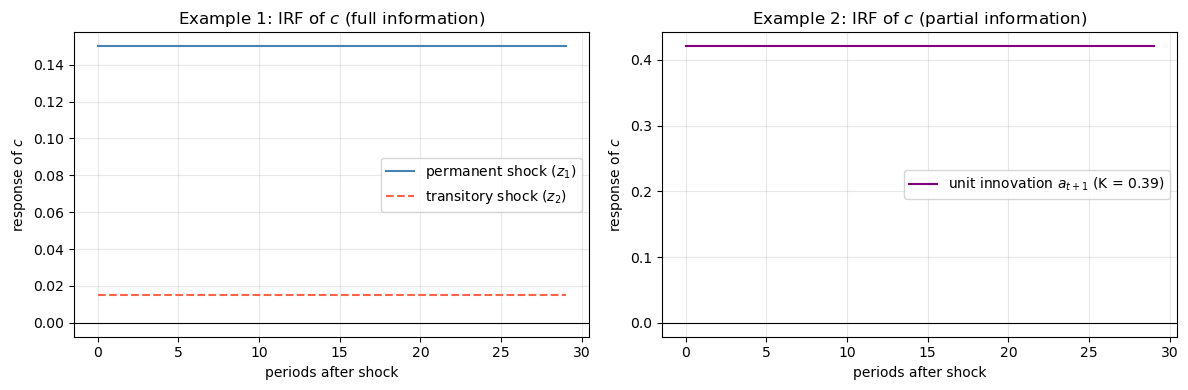
Fig. 80.1 Consumption impulse responses in the two examples#
Note
The impulse responses have the “box” shape characteristic of the LQ permanent income model: once a shock occurs, consumption shifts permanently to a new level and stays there.
80.2.9. Spreading consumption cross sections#
The unit root in consumption (Representation 2) causes the cross-section variance of consumption to grow linearly with age.
Consider a continuum of ex ante identical households born at \(t = 0\).
Each household \(i\) has the same preferences and the same stochastic income process, but faces idiosyncratic shocks \(w_{t+1}^i\).
Let all households start from the same initial conditions \(c_0^i = c_0\) and \(z_0^i\).
From (80.16), household \(i\)’s consumption follows
Since the \(w^i_{t+1}\) are independent across agents,
In the two-factor model, \(h\) is a \(1 \times 2\) row vector so \(hh'\) is a positive scalar equal to \(\sigma_1^2 + (1-\beta)^2\sigma_2^2\).
The cross-section variance of consumption grows like \(t\).
# Simulate cross-section spreading
rng = np.random.default_rng(42)
N      = 5000       # number of agents
T_sim  = 80         # number of periods

h_vec  = (1 - β) * (M @ C_check)   # shape (1, 2), then flatten
h_vec  = h_vec.flatten()            # h = [h1, h2]

c = np.zeros((N, T_sim + 1))       # consumption paths
# initialise all agents at c_0 = 0 (demeaned)
for t in range(T_sim):
    eps = rng.standard_normal((N, 2))    # N draws of 2D shock
    dc  = eps @ h_vec              # shape (N,)
    c[:, t+1] = c[:, t] + dc

# Cross-section variance at each date
var_c  = np.var(c, axis=0)
theory = np.arange(T_sim + 1) * np.dot(h_vec, h_vec)

fig, ax = plt.subplots()
ax.plot(var_c,  label='simulated cross-section variance', linewidth=2)
ax.plot(theory, label=r'theoretical: $t \cdot h h^\prime$',
        linestyle='--', color='tomato')
ax.set_xlabel('period $t$')
ax.set_ylabel('cross-section variance of $c$')
ax.legend()
ax.grid(alpha=0.3)
plt.show()
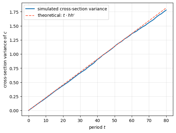
Fig. 80.2 Spreading consumption cross sections#
80.2.10. A “borrowers and lenders” closed economy (Bewley model)#
Up to now we have set \(R = \beta^{-1}\) and taken it as determined outside the model (“small open economy”).
Following ideas of [Bewley, 1977], we can construct a closed economy in which \(R = \beta^{-1}\) is an equilibrium outcome.
Environment. A continuum of measure one of consumers, indexed by \(i \in [0,1]\), trade a risk-free one-period bond with price \(\beta\).
All consumers have the same preferences and the same stochastic income process, but face idiosyncratic income shocks.
Initial bond positions are zero: \(b_0^i = 0\) for all \(i\).
Initial endowment states \(z_0^i\) are independent draws from the stationary distribution of (80.3).
Individual decisions. From (80.10), with \(b_0^i = 0\), agent \(i\)’s time-0 consumption is
For \(t \geq 1\), from (80.16):
Market clearing. Let \(Y\) denote the stationary mean of the cross-section average of non-financial income. Integrating (80.27) over all agents:
because the continuum of idiosyncratic shocks averages out.
For future periods, integrating (80.28):
The goods market clears at every date at constant aggregate consumption equal to \(Y\).
The bond market clears at zero net supply each period. Thus \(R = \beta^{-1}\) is an equilibrium outcome: we have constructed a Bewley model.
Cross-section inequality. While the cross-section mean of consumption is constant, the cross-section variance grows without bound according to (80.26). Initial differences in endowment draws \(z_0^i\) create permanent differences in consumption levels, and idiosyncratic shocks create ongoing divergence.
# Verify Bewley market clearing via simulation
# We use an online (Welford) accumulator for mean and variance so that we never
# store the full NxT consumption array in memory.
rng = np.random.default_rng(0)
N_bew  = 10000    # agents - enough to illustrate the law of large numbers
T_bew  = 60

# Draw initial z^i_0; z1 is a random walk so its stationary distribution is
# degenerate - we draw from a distribution with std 1 for illustration.
z0_i   = rng.standard_normal((N_bew, 2)) * np.array([1.0, σ2])
c0_i   = ((1 - β) * (M @ z0_i.T)).flatten()   # shape (N_bew,)

# Online accumulation: propagate c_t across agents without storing all paths.
mean_c = np.zeros(T_bew + 1)
var_c2 = np.zeros(T_bew + 1)
mean_c[0] = c0_i.mean()
var_c2[0] = c0_i.var()

c_now = c0_i.copy()
for t in range(T_bew):
    eps    = rng.standard_normal((N_bew, 2))
    c_now  = c_now + eps @ h_vec
    mean_c[t + 1] = c_now.mean()
    var_c2[t + 1] = c_now.var()

# Keep c0_i available for the complete-markets figure below
c_bew_t0 = c0_i

fig, axes = plt.subplots(1, 2, figsize=(12, 4))

axes[0].plot(mean_c, linewidth=2, color='steelblue')
axes[0].axhline(mean_c[0], linestyle='--', color='tomato', label='initial mean')
axes[0].set_title('Cross-section mean of $c$ (Bewley economy)')
axes[0].set_xlabel('period $t$')
axes[0].set_ylabel('mean consumption')
axes[0].legend()
axes[0].grid(alpha=0.3)

axes[1].plot(var_c2, linewidth=2, color='steelblue', label='simulated variance')
axes[1].set_title('Cross-section variance of $c$ (Bewley economy)')
axes[1].set_xlabel('period $t$')
axes[1].set_ylabel('variance of consumption')
axes[1].legend()
axes[1].grid(alpha=0.3)

plt.tight_layout()
plt.show()
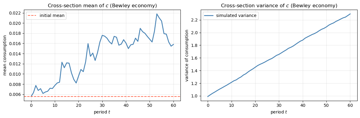
Fig. 80.3 Bewley economy cross-section moments#
An inefficiency. Because each consumer dislikes variation of consumption over time, each consumer would prefer a completely smoothed stream \(c_t^i = c_0^i\) for all \(t\). Such an allocation is feasible (the cross-section average of income is constant), and it is Pareto superior to the incomplete-markets equilibrium. The next section describes the complete-markets allocation that achieves this.
80.2.11. Consumption smoothing with complete markets#
We replace the single bond with a complete set of Arrow securities. The budget constraint becomes
where \(q(z_{t+1}|z_t)\) is the pricing kernel for one-period state-contingent claims and \(b_t(z_{t+1})\) is the household’s portfolio of Arrow securities chosen at \(t\).
Equilibrium pricing kernel. We conjecture (and verify) that the equilibrium pricing kernel is
where \(\phi(z_{t+1}|z_t)\) is the transition density of \(z\). This kernel prices a one-period risk-free bond at \(\beta\), so \(R = \beta^{-1}\), consistent with the incomplete-markets equilibrium.
Constant consumption conjecture. We conjecture that the equilibrium delivers each consumer \(i\) a constant consumption level:
where \(c_0^i = (1-\beta)\,\check{G}(I-\beta\check{A})^{-1} z_0^i\) is the consumer’s time-0 consumption in the incomplete-markets economy.
Supporting portfolio. The state-contingent debt that supports constant consumption is
Note that indebtedness depends only on the current Markov state \(z_t\), not on the history of earlier states. This absence of history dependence reflects the complete risk sharing attained under complete markets.
Substituting the pricing kernel (80.31) and the portfolio conjecture (80.33) into the budget constraint (80.30) and using the law of iterated expectations confirms that the budget constraint simplifies to \(c_t = \bar{c}^i\) in every state and period.
Cross-section implications. Under complete markets:
The cross-section distribution of consumption is time-invariant.
Consumer \(i\)’s rank in the consumption distribution is fixed forever.
A lucky initial draw \(z_0^i\) manifests itself as perpetually high consumption \(\bar{c}^i\) and lower indebtedness \(b(z_t^i, \bar{c}^i)\) across all future states.
This contrasts sharply with the incomplete-markets Bewley economy, where the cross-section variance of consumption grows without bound.
# Illustrate: complete vs incomplete markets consumption distributions over time
rng = np.random.default_rng(1)
N_cm = 5000
T_cm = 50

# Initial consumption draws (same as Bewley economy)
c0_cm = c_bew_t0[:N_cm]   # initial consumption draws from the Bewley cell above

# Incomplete markets: consumption evolves (random walk)
c_inc = np.zeros((N_cm, T_cm + 1))
c_inc[:, 0] = c0_cm
for t in range(T_cm):
    eps = rng.standard_normal((N_cm, 2))
    c_inc[:, t+1] = c_inc[:, t] + eps @ h_vec

# Complete markets: consumption stays constant
c_comp = np.tile(c0_cm[:, np.newaxis], T_cm + 1)

fig, axes = plt.subplots(1, 2, figsize=(12, 4))

for t_plot, color in zip([0, 10, 30, 50], ['steelblue', 'orange', 'tomato', 'purple']):
    axes[0].hist(c_inc[:, t_plot], bins=60, alpha=0.4,
                 label=f't = {t_plot}', color=color, density=True)
axes[0].set_title('Incomplete markets:\ncross-section distribution of $c$')
axes[0].set_xlabel('$c$')
axes[0].legend(fontsize=9)
axes[0].grid(alpha=0.3)

for t_plot, color in zip([0, 10, 30, 50], ['steelblue', 'orange', 'tomato', 'purple']):
    axes[1].hist(c_comp[:, t_plot], bins=60, alpha=0.4,
                 label=f't = {t_plot}', color=color, density=True)
axes[1].set_title('Complete markets:\ncross-section distribution of $c$')
axes[1].set_xlabel('$c$')
axes[1].legend(fontsize=9)
axes[1].grid(alpha=0.3)

plt.tight_layout()
plt.show()
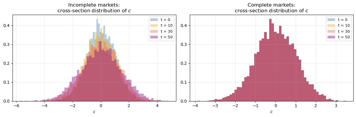
Fig. 80.4 Complete vs incomplete markets consumption distributions#
Note
Under complete markets the histogram stays the same across all \(t\) (distributions overlap perfectly), while under incomplete markets the distribution spreads out over time.
Connecting Part A to Part B. Part A derived optimal consumption rules for a consumer who fully trusts his stochastic income model. Part B relaxes that assumption: the consumer fears that the model is misspecified and therefore seeks decision rules that are robust to plausible alternatives. We will see that the optimal robust rule takes the same form as the Part A rule, but under a distorted model of the income process that looks more persistent than the approximating one.
80.3. Part B: a robust permanent income model#
80.3.1. Introduction#
Part B studies a consumer who distrusts his specification of the stochastic process governing his labor income. The model is due to Hansen, Sargent, and Tallarini (1999) (HST) [Hansen et al., 1999], who estimated it on US quarterly consumption and investment data.
A consumer who fears model misspecification engages in a form of precautionary savings that is distinct from the usual precautionary motive (which requires a convex marginal utility).
Here, the precautionary motive arises because the consumer wants to protect against misspecification of the conditional means of income shocks, and it operates even with quadratic preferences.
HST showed an important observational equivalence result: for quantities \((c_t, i_t)\) alone, a concern for robustness is indistinguishable from an increase in impatience (a decrease in \(\beta\)).
We develop this result carefully below.
Outline of Part B:
State the HST model (planner’s Bellman equation with robustness).
Solve the \(\sigma = 0\) benchmark.
Prove observational equivalence (Theorem 1 and Theorem 2).
Interpret the result using distorted expectations from a Stackelberg multiplier game.
Illustrate frequency-domain and detection-error-probability aspects.
Evaluate the robustness of alternative decision rules.
80.3.2. The HST model#
HST’s model features a planner with preferences over consumption streams \(\{c_t\}\), mediated through service streams \(\{s_t\}\). Let \(b\) be a preference shifter (utility bliss point).
The Bellman equation for the robust planner is
subject to the household technology, capital accumulation, endowment dynamics, and the state law:
Here \(^*\) denotes the next-period value; \(c\) is consumption; \(s\) is the scalar service measure; \(h\) is a habit stock; \(k\) is the capital stock; \(i\) is investment; \(d\) is an endowment/technology shock; \(b\) is a preference shock (bliss-point shifter, distinct from the bond/debt variable \(b_t\) used in Part A); \(\epsilon^* \sim \mathcal{N}(0,I)\) is the baseline shock; and \(w^*\) is a distortion to the conditional mean of \(\epsilon^*\) chosen by an evil agent.
The penalty parameter \(\theta > 0\) governs the consumer’s concern about robustness. We use the transformation
so \(\sigma = 0\) corresponds to no robustness concern and \(\sigma < 0\) to an increasing concern.
Household technology. When \(\lambda > 0\) and \(\delta_h \in (0,1)\), the technology (80.35) accommodates habit persistence (positive \(\lambda\)) or durability. The stock \(h_t\) is a geometric weighted average of current and past consumption.
Production technology. Equation \(c_t + k_t = Rk_{t-1} + d_t\) with \(R = \delta_k + \gamma\) combines capital accumulation with a linear production technology. \(R\) is the physical gross return on capital.
State vector. Let \(x_t' = [h_{t-1},\, k_{t-1},\, z_t']\). There is a set of state transition equations:
where \(u_t = c_t\) and \(w_{t+1}\) is the distortion to the conditional mean of \(\epsilon_{t+1}\).
HST’s calibration. HST estimated the model on U.S. quarterly data (1970Q1-1996Q3) using nondurables plus services for consumption and durable consumption plus gross private investment for investment. Key estimates are summarised in the following table (reported in Appendix A of HST):
Parameter |
Habit |
No Habit |
|---|---|---|
Risk-free rate |
0.025 |
0.025 |
\(\beta\) |
0.997 |
0.997 |
\(\delta_h\) |
0.682 |
— |
\(\lambda\) |
2.443 |
0 |
\(\alpha_1\) |
0.813 |
0.900 |
\(\alpha_2\) |
0.189 |
0.241 |
\(\phi_1\) |
0.998 |
0.995 |
\(\phi_2\) |
0.704 |
0.450 |
\(2 \times \log L\) |
779.05 |
762.55 |
HST imposed \(\beta R = 1\) and \(\delta_k = 0.975\), so \(\gamma\) is pinned down once \(\beta\) is estimated. An annual real interest rate of 2.5% corresponds to \(\beta = 0.997\).
80.3.3. Solution when \(\sigma = 0\)#
When \(\sigma = 0\) the objective reduces to
Formulating a Lagrangian and deriving first-order conditions yields:
Here \(\mu_{st}\) is the marginal valuation of consumption services, which summarises the endogenous state variables \(h_{t-1}\) and \(k_{t-1}\). Equation (80.38) (last line) implies \(\mathbb{E}_t\mu_{c,t+1} = (\beta R)^{-1}\mu_{ct}\), so \(\mu_{st}\) satisfies a martingale representation when \(\beta R = 1\):
for some vector \(\nu\). Solving forward and substituting gives
where
and \(\tilde\delta_h = (\delta_h + \lambda)/(1+\lambda)\).
In the widely-studied special case \(\lambda = \delta_h = 0\), so \(s_t = c_t\) and \(\mu_{st} = b_t - c_t\), the marginal propensity to consume out of non-human wealth \(Rk_{t-1}\) equals that out of human wealth \(\sum_{j=0}^{\infty}R^{-j}\mathbb{E}_t d_{t+j}\), a well-known feature of the LQ model.
Representing \(\nu\) in matrix form. The formula for \(\mu_{st}\) can be written as \(\mu_{st} = M_s x_t\) where \(x_t\) follows (80.36). It follows that
The scalar \(\alpha\) plays a central role in the observational equivalence result below.
80.3.4. Observational equivalence#
80.3.4.1. Theorem 1: HST observational equivalence#
The key result of HST is:
Theorem 1 (Observational Equivalence, I). Fix all parameters except \((\sigma, \beta)\). Suppose \(\beta R = 1\) when \(\sigma = 0\). There exists \(\underline\sigma < 0\) such that for any \(\sigma \in (\underline\sigma, 0)\), the optimal consumption-investment plan for \((0,\beta)\) is also chosen by a robust decision maker with parameters \((\sigma, \hat\beta(\sigma))\), where
and \(\hat\beta(\sigma) < \beta\).
Intuition. Since \(R > 1\) and \(\alpha^2 > 0\), a more negative \(\sigma\) (stronger robustness concern) lowers \(\hat\beta\). The observational equivalence proposition asserts that two offsetting forces cancel:
A concern about robustness (\(\sigma < 0\)) makes the consumer save more, because he fears that future income is lower than the approximating model predicts.
Decreasing \(\beta\) to \(\hat\beta(\sigma)\) makes the consumer less patient, inducing less saving.
When these two forces are balanced according to (80.43), the consumption and investment quantities are identical across \((\sigma, \hat\beta(\sigma))\) pairs.
80.3.4.2. Proof sketch#
When \(\beta R = 1\) and \(\sigma = 0\), the marginal utility \(\mu_{st}\) obeys the martingale
where \(\tilde\epsilon_t\) is scalar i.i.d.\ with mean zero and unit variance. Activating robustness (\(\sigma < 0\)) means the evil agent solves
making the worst-case model for \(\mu_{st}\):
For the allocation to remain the same, we require the robust Euler equation \(\hat\beta R\,\hat{\mathbb{E}}_t\mu_{s,t+1} = \mu_{st}\) to hold under the worst-case model, which gives
The evil agent’s Bellman equation (a pure forecasting problem) yields
where \(P(\hat\beta)\) solves the scalar Bellman equation:
Solving (80.46)-(80.48) for \(\hat\beta\) gives exactly (80.43). \(\square\)
80.3.5. Observational equivalence: numerical illustration#
# Observational equivalence locus: β_hat(σ) = 1/R + σα^2 / (R-1)
# HST benchmark values
β0    = 0.997          # benchmark discount factor
R0    = 1.0 / β0       # gross interest rate
α2_vals = [0.005, 0.015, 0.030]   # three values of α^2 for illustration

σ_grid = np.linspace(-0.002, 0.0, 400)

fig, ax = plt.subplots()
for α2 in α2_vals:
    β_hat = 1/R0 + σ_grid * α2 / (R0 - 1)
    ax.plot(σ_grid, β_hat, label=rf'$\alpha^2 = {α2}$')

ax.axhline(β0, linestyle=':', color='grey', linewidth=1, label=r'$\beta_0 = 0.997$')
ax.axvline(0,  linestyle=':', color='grey', linewidth=1)
ax.set_xlabel(r'$\sigma = -\theta^{-1}$ (robustness parameter)')
ax.set_ylabel(r'$\hat\beta(\sigma)$')
ax.legend()
ax.grid(alpha=0.3)
plt.show()
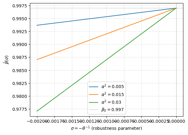
Fig. 80.5 Observational equivalence locus#
Note
Each point on a locus is observationally equivalent (given only data on \((c_t, i_t)\)) to the benchmark \((\sigma=0, \beta_0)\). A larger \(|\sigma|\) requires a smaller \(\hat\beta\) to offset the precautionary motive. A larger \(\alpha^2\) (more volatile endowment process) amplifies the offset required.
80.3.6. Precautionary savings interpretation#
The consumer’s concern about model misspecification activates a particular kind of precautionary savings motive that underlies the observational equivalence proposition.
How it works. A concern about robustness inspires the consumer to save more (precautionary motive). Decreasing \(\beta\) induces the consumer to save less (impatience). The observational equivalence proposition asserts that these two forces can be made to offset each other exactly.
The special case \(\lambda = \delta_h = 0\). Here \(s_t = c_t\) and the consumption rule is
The marginal propensity to consume out of non-human wealth \(Rk_{t-1}\) equals that out of human wealth \(\mathbb{E}_t\sum R^{-j}d_{t+j}\). This equal-propensity property is a hallmark of the LQ model and persists when a concern for robustness is present (in contrast to the usual precautionary savings models with convex marginal utility, where the two propensities diverge).
Theorem 1 offset. Theorem 1 says that with \(\sigma < 0\), the observationally equivalent \(\hat\beta\) satisfies \(\hat\beta < \beta\). If the starting point has \(\beta R = 1\), then \(\hat\beta R < 1\). For a non-robust consumer with discount factor \(\hat\beta\) at the same interest rate, the Euler equation implies \(\mathbb{E}_t c_{t+1} < c_t\): expected consumption declines over time.
This downward drift is the impatience offset in Theorem 1. It cancels the robust consumer’s precautionary-savings motive, leaving the consumption and investment quantities unchanged. The upward-drift comparison appears below in Theorem 2, which asks the reverse observational equivalence question.
Comparison with classical precautionary savings. The classical precautionary motive (see Leland 1968 and Miller 1974) arises because:
This channel requires convexity of marginal utility and is absent with quadratic preferences. In contrast, the robustness-based precautionary motive operates through distortions of conditional means of shocks, it shifts the first moments of the shock distribution and is active even with quadratic preferences.
# Illustrate the Theorem 1 offset: lower β_hat at fixed R
# In the special case λ = δ_h = 0:
# With β0 R = 1, Theorem 1 gives β_hat < β0 and hence β_hat R < 1
# Euler equation: E_t c_{t+1} = (β_hat R) c_t  -> downward drift

β_vals  = [0.990, 0.993, 0.995]     # σ < 0 <-> β_hat < β0 in Theorem 1
R_fixed = 1 / 0.997
T_plot  = 40

fig, ax = plt.subplots()
t_grid = np.arange(T_plot + 1)
c0     = 1.0
for β_hat_i in β_vals:
    drift = (β_hat_i * R_fixed) ** t_grid
    label = rf'$\hat\beta = {β_hat_i}$, $\hat\beta R = {β_hat_i*R_fixed:.4f}$'
    ax.plot(t_grid, c0 * drift, label=label)

ax.axhline(c0, linestyle=':', color='grey', linewidth=1,
           label=r'$\beta_0 R = 1$ (benchmark)')
ax.set_xlabel('period $t$')
ax.set_ylabel(r'$E_0 c_t / c_0$')
ax.legend(fontsize=9)
ax.grid(alpha=0.3)
plt.show()
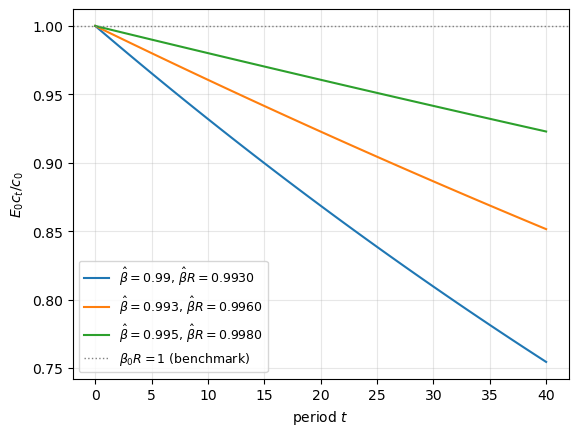
Fig. 80.6 Expected consumption profile under Theorem 1 discount-factor offsets#
80.3.7. Observational equivalence and distorted expectations#
The observational equivalence result can be interpreted using a Stackelberg multiplier game. After the minimising evil agent has committed to a distortion process \(\{w_{t+1}\}\), the maximising consumer faces the following worst-case law of motion for the state \(X_t\):
The consumer forms expectations of future income using the distorted transition matrix \(A - BF + CK\) rather than the approximating transition matrix \(A - BF\).
The distorted expectations operator \(\hat{\mathbb{E}}_t\) satisfies
Observational equivalence requires that the modified human-wealth formula
equals its benchmark counterpart \(\Psi_4 \sum_{j=0}^{\infty} R^{-j} \mathbb{E}_t d_{t+j}\). This is achieved by a mutual adjustment of the coefficients \(\hat\Psi_j\) (via \(\hat\beta\)) and the distorted expectation operator \(\hat{\mathbb{E}}_t\) (via \(\sigma\)).
Distorted endowment process. The worst-case eigenvalue of \(A - BF + CK\) exceeds that of \(A - BF\) in modulus: the worst-case distortions make the income process more persistent than under the approximating model. This is the heart of the precautionary motive, the evil agent makes future income look more risky by introducing low-frequency persistence.
# Illustrate how worst-case model makes endowment process more persistent
# We work with a simplified scalar AR(1) version for illustration:
#   d_{t+1} = ρ d_t + σ_d ε_{t+1}      (approximating model)
# The worst-case distortion increases the effective AR coefficient

ρ_approx = 0.80   # AR coefficient under approximating model
σ_d      = 0.10   # endowment shock std

# Under worst-case model: effective AR coefficient = ρ + α*K(σ, β_hat)
# Here we show how the worst-case AR coefficient varies with |σ|
σ_rob_vals = [0.0, -0.0001, -0.0003, -0.0005]
T_irf      = 30

fig, ax = plt.subplots()
for σ_rob in σ_rob_vals:
    # α K ~= |σ| * P * α^2 / (1 - |σ| * α^2 * P) - simplified scalar version
    # For illustration, use a linear approximation: Δρ ~= -σ * α^2 * const
    α2_scal  = 0.01
    Δρ       = -σ_rob * α2_scal * 2.0    # heuristic scaling for illustration
    ρ_wc     = ρ_approx + Δρ
    irf      = ρ_wc ** np.arange(T_irf)
    if σ_rob == 0.0:
        ax.plot(irf, linewidth=2.5, linestyle='-',
                label=rf'approx. model ($\sigma = 0$, $\rho = {ρ_approx}$)')
    else:
        ax.plot(irf, linestyle='--',
                label=rf'worst-case ($\sigma = {σ_rob}$, $\rho_{{wc}} \approx {ρ_wc:.4f}$)')

ax.set_xlabel('periods after shock')
ax.set_ylabel('impulse response of $d_t$')
ax.legend(fontsize=9)
ax.grid(alpha=0.3)
plt.show()
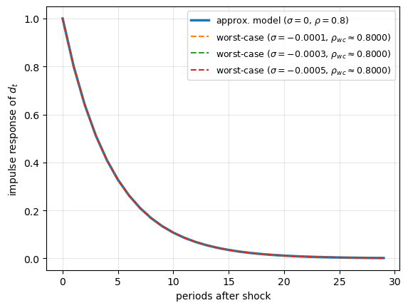
Fig. 80.7 Worst-case model makes endowment more persistent#
80.3.8. Frequency domain interpretation#
The LQ permanent income framework has a natural frequency-domain interpretation:
The consumer’s concave utility makes him dislike high-frequency fluctuations in consumption. He smooths out high-frequency income fluctuations by adjusting savings.
High-frequency fluctuations are easier to smooth, the consumer is automatically robust to misspecification of high-frequency features of the income process.
Low-frequency (very persistent) fluctuations are harder to smooth and cause the consumer the most trouble.
In the frequency-domain notation of HST, the transfer function from shocks \(\epsilon_t\) to the target \(s_t - b_t\) is \(G(\zeta)\), and the frequency decomposition of the \(H_2\) criterion is
The integrand \(G'G\) is largest at low frequencies \(\omega \approx 0\), the consumer’s welfare is most sensitive to low-frequency income variability.
Recognising this, the evil agent concentrates the worst-case distortions at low frequencies. The distortion process has spectral density \(W(\zeta)' W(\zeta)\) that is concentrated near \(\omega = 0\). The variance of the worst-case shocks grows as \(|\sigma|\) increases.
# Illustrate frequency concentration of worst-case shocks
# We plot a stylised version of trace[W(ζ)'W(ζ)] vs frequency

ω_grid = np.linspace(-np.pi, np.pi, 500)

# Approximating model: flat spectrum (i.i.d. shocks)
spectrum_approx = np.ones_like(ω_grid)

# Worst-case shocks: power concentrated at low frequencies
# Model as a low-pass spectrum W(ω) ~ 1/(ω^2 + κ^2)
def low_pass(ω, κ, scale):
    return scale / (ω**2 + κ**2)

fig, axes = plt.subplots(1, 2, figsize=(12, 4))

# Left panel: criterion G'G (low-frequency dominance)
G_sq = 1.0 / (np.abs(np.exp(1j * ω_grid) - 0.95)**2 + 0.01)
G_sq = G_sq / G_sq.max()
axes[0].plot(ω_grid, G_sq, color='steelblue', linewidth=2)
axes[0].set_title(r"Stylised $G(\zeta)'G(\zeta)$ vs frequency $\omega$")
axes[0].set_xlabel(r'frequency $\omega$')
axes[0].set_ylabel(r'$G(\zeta)^\prime G(\zeta)$')
axes[0].set_xlim(-np.pi, np.pi)
axes[0].grid(alpha=0.3)
axes[0].text(0, 0.5, 'Low-frequency\ndominance', ha='center', fontsize=10, color='steelblue')

# Right panel: worst-case shock spectra for two values of |σ|
for σ_abs, kap, scale in [(0.0001, 0.02, 0.8), (0.00005, 0.02, 0.4)]:
    W_sq = low_pass(ω_grid, kap, scale) + 0.01
    W_sq = W_sq / W_sq.max() * σ_abs / 0.0001
    axes[1].plot(ω_grid, W_sq,
                 label=rf'$|\sigma| = {σ_abs}$')
axes[1].set_title(r"Stylised $\operatorname{tr}[W(\zeta)'W(\zeta)]$ vs frequency")
axes[1].set_xlabel(r'frequency $\omega$')
axes[1].set_ylabel(r'$\operatorname{tr}[W^\prime W]$')
axes[1].set_xlim(-np.pi, np.pi)
axes[1].legend()
axes[1].grid(alpha=0.3)

plt.tight_layout()
plt.show()
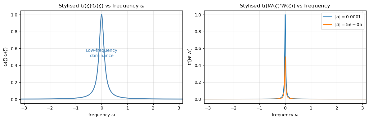
Fig. 80.8 Worst-case distortions concentrate at low frequencies#
80.3.9. Detection error probabilities#
A natural way to discipline the choice of \(\sigma\) (or \(\theta\)) is to ask: how difficult would it be to statistically distinguish the approximating model from the worst-case model?
For a sample of length \(T\), one can use a log-likelihood ratio test to compare the two hypotheses. The detection error probability (DEP) is the probability of making the wrong decision using the log-likelihood ratio statistic when one does not know which model generated the data. Specifically:
When \(\sigma = 0\) the two models are identical and DEP \(= 0.5\). As \(|\sigma|\) increases the models diverge and the DEP falls toward zero.
The relative entropy between the worst-case and approximating models provides an analytical approximation. For the scalar version of the problem, the Kullback-Leibler divergence between the two Gaussian models over \(T\) periods is approximately:
# Illustrate detection error probabilities (scalar stylised version)
# We compute relative entropy approximation and convert to DEP

T_sample = 107        # HST sample length (1970Q1 - 1996Q3)
α2_val   = 0.01       # representative α^2 value
R_dep    = 1.0 / 0.997

# For each σ compute: K(σ,β_hat) from worst-case multiplier, then Δ, then DEP
def compute_dep(σ_val, α2, R, T):
    """
    Compute detection error probability for a given σ.
    Uses a simplified scalar approximation.
    """
    if σ_val == 0.0:
        return 0.5
    β_hat = 1.0 / R + σ_val * α2 / (R - 1)
    if β_hat <= 0:
        return 0.0

    # Scalar Bellman equation for P(β_hat)
    disc  = (β_hat - 1 + σ_val * α2)**2 + 4 * σ_val * α2
    if disc < 0:
        return np.nan
    P_val = (β_hat - 1 + σ_val * α2 + np.sqrt(disc)) / (-2 * σ_val * α2)

    # Worst-case gain K
    K_val  = σ_val * α2 * P_val / (1 - σ_val * α2 * P_val)

    # KL divergence (one-sided) approximation per period: 0.5 * K^2 * α^2
    kl_per = 0.5 * K_val**2 * α2
    kl_T   = kl_per * T

    # DEP ~= Φ(-sqrt(KL_T / 2)) where Φ is standard normal CDF
    dep    = norm.cdf(-np.sqrt(kl_T / 2))
    return dep

σ_dep_grid = np.linspace(-0.002, 0, 200)
dep_vals   = np.array([compute_dep(s, α2_val, R_dep, T_sample)
                       for s in σ_dep_grid])

fig, ax = plt.subplots()
ax.plot(σ_dep_grid, dep_vals, linewidth=2, color='steelblue')
ax.axhline(0.5, linestyle=':', color='grey', linewidth=1, label='DEP = 0.5 at σ = 0')
ax.axhline(0.3, linestyle='--', color='tomato', linewidth=1, label='DEP = 0.3 (plausible threshold)')
ax.axhline(0.2, linestyle='--', color='orange', linewidth=1, label='DEP = 0.2')
ax.set_xlabel(r'$\sigma$ (robustness parameter)')
ax.set_ylabel('detection error probability')
ax.legend()
ax.grid(alpha=0.3)
plt.show()
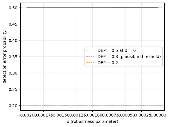
Fig. 80.9 Detection error probabilities#
Note
HST suggested that a DEP above 0.2 is “plausible”, meaning the models are still hard enough to distinguish statistically that a concern for robustness is warranted. Values of \(\sigma\) corresponding to DEP \(\geq 0.2\) define a set of plausible worst-case models.
80.3.10. Robustness of decision rules#
To evaluate whether robust decision rules perform better than the non-robust rule when the data are generated by a distorted model, define the payoff when the decision rule is designed for robustness parameter \(\sigma_2\) and the data are generated by the distorted model associated with \(\sigma_1\):
where the state evolves under decision rule \(F(\sigma_2)\) and worst-case shocks \(K(\sigma_1)\):
For \(\sigma_1 = 0\) (approximating model generates data), the non-robust rule (\(\sigma_2 = 0\)) is optimal by construction. As \(\sigma_1\) decreases (the data are generated by increasingly distorted models), the payoff of the \(\sigma_2 = 0\) rule deteriorates faster than that of robust rules.
# Illustrate robustness payoff comparison (scalar stylised version)
# π(σ1; σ2) measures performance of rule σ2 when model σ1 generates data

α2_rob   = 0.01
R_rob    = 1.0 / 0.997
β_rob    = 0.997
σ2_vals  = [0.0, -0.0004, -0.0008]   # three decision-rule robustness levels

σ1_grid  = np.linspace(-0.0010, 0.0, 300)

def payoff_approx(σ1, σ2, α2, β, R):
    """
    Approximate payoff π(σ1; σ2) in a stylised scalar version.
    Captures the key qualitative pattern from HST.
    """
    # Effective drift under (F(σ2), K(σ1)):
    β_hat2 = 1.0/R + σ2 * α2 / (R - 1) if σ2 != 0 else β
    β_hat1 = 1.0/R + σ1 * α2 / (R - 1) if σ1 != 0 else β

    # K for σ1
    if σ1 == 0.0:
        K1 = 0.0
    else:
        disc = (β_hat1 - 1 + σ1*α2)**2 + 4*σ1*α2
        if disc < 0: return np.nan
        P1 = (β_hat1 - 1 + σ1*α2 + np.sqrt(disc)) / (-2*σ1*α2)
        K1 = σ1 * α2 * P1 / (1 - σ1*α2*P1)

    # Effective persistence of state under (F(σ2), K(σ1))
    ρ_eff  = 0.85 + K1 * np.sqrt(α2)   # simplified
    if abs(ρ_eff) >= 1.0:
        return np.nan

    # Lyapunov variance of state
    var_x  = α2 / (1 - ρ_eff**2)

    # Per-period loss scales with variance of state
    loss   = -var_x * (1.0 + 0.5 * abs(σ2) / 0.001)
    return loss

fig, ax = plt.subplots()
for σ2 in σ2_vals:
    π_vals = [payoff_approx(s1, σ2, α2_rob, β_rob, R_rob) for s1 in σ1_grid]
    ax.plot(σ1_grid, π_vals, label=rf'$\sigma_2 = {σ2}$ (rule)')

ax.set_xlabel(r'$\sigma_1$ (data-generating distortion)')
ax.set_ylabel(r'$\pi(\sigma_1;\,\sigma_2)$')
ax.legend(fontsize=9)
ax.grid(alpha=0.3)
plt.show()
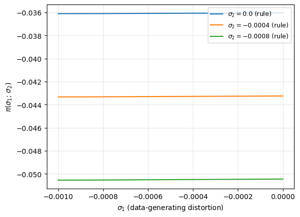
Fig. 80.10 Payoff of robust vs non-robust rules#
Note
The function payoff_approx is a reduced-form scalar analogue of the full HST matrix
calculation. It keeps the same comparison – fix a data-generating distortion \(\sigma_1\)
and compare rules indexed by \(\sigma_2\) – but it is not calibrated to reproduce HST’s
numerical payoffs. The figure should be read as a qualitative payoff comparison.
Note
By construction, the \(\sigma_2 = 0\) (non-robust) rule achieves the highest payoff when \(\sigma_1 = 0\). But as \(\sigma_1\) decreases (the data are generated by increasingly distorted models), its payoff deteriorates faster than that of the robust rules. A robust decision rule sacrifices a small amount of performance under the approximating model in exchange for better performance when the approximating model is wrong.
80.3.11. Another observational equivalence result#
Theorem 2 (Observational Equivalence, II). Fix all parameters except \((\sigma,\beta)\). Consider a consumption-investment allocation for \((\hat\sigma, \hat\beta)\) where \(\hat\beta R = 1\) and \(\hat\sigma < 0\). Then there exists \(\tilde\beta > \hat\beta\) such that the \((\hat\sigma, \hat\beta)\) allocation also solves the \((0, \tilde\beta)\) problem.
Interpretation. Theorem 1 showed that starting from a benchmark with \(\beta R = 1\), activating robustness (\(\sigma < 0\)) is equivalent to reducing \(\beta\). Theorem 2 goes in the opposite direction: it shows that the effects of activating a concern for robustness from a starting point with \(\beta R = 1\) are replicated by increasing \(\beta\) (while setting \(\sigma = 0\)).
In other words, when \(\beta R = 1\), a concern for robustness operates like an increase in the discount factor, pushing \(\beta R > 1\) and imparting an upward drift to the expected consumption profile.
Proof. With \(\hat\beta R = 1\) and \(\hat\sigma < 0\), the robust Euler equation implies
One seeks \(\tilde\beta > \hat\beta\) and \(\sigma = 0\) such that the same allocation solves the non-robust problem with discount factor \(\tilde\beta\). The key step is to observe that the worst-case distortion \(K(\hat\sigma, \hat\beta)\) introduces a drift in the marginal utility process that is equivalent to the drift produced by raising the discount factor above \(\hat\beta\). Equating the two drifts and solving the scalar Bellman equation for \(K\) yields
The solution satisfies \(\tilde\beta > \hat\beta\) when \(\hat\sigma < 0\). \(\square\)
# Compute the Theorem 2 equivalence: β_tilde(σ_hat) vs σ_hat
# Starting from β_hat R = 1 and σ_hat < 0

β_hat_val  = 0.997     # β_hat satisfying β_hatR = 1
α2_th2     = 0.01

σ_hat_grid = np.linspace(-0.001, 0.0, 300)

def β_tilde(σ_hat, β_hat, α2):
    """Theorem 2 formula for β_tilde."""
    disc = 1 - 4 * β_hat * (1 + σ_hat * α2) / (1 + β_hat)**2
    if np.any(disc < 0):
        disc = np.maximum(disc, 0)
    return β_hat * (1 + β_hat) / (2 * (1 + σ_hat * α2)) * (1 + np.sqrt(disc))

β_tilde_vals = β_tilde(σ_hat_grid, β_hat_val, α2_th2)

fig, ax = plt.subplots()
ax.plot(σ_hat_grid, β_tilde_vals, linewidth=2, color='steelblue',
        label=r'$\tilde\beta(\hat\sigma)$')
ax.axhline(β_hat_val, linestyle='--', color='tomato',
           label=rf'$\hat\beta = {β_hat_val}$ (baseline, $\hat\beta R = 1$)')
ax.set_xlabel(r'$\hat\sigma$ (robustness parameter)')
ax.set_ylabel(r'$\tilde\beta$')
ax.legend()
ax.grid(alpha=0.3)
plt.show()
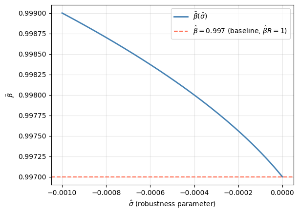
Fig. 80.11 Theorem 2 observational equivalence locus#
80.3.12. A robust LQ Bewley model#
We now synthesise Parts A and B by embedding the Bewley economy of Part A into the HST framework and applying the observational equivalence theorem. This constructs a family of robust Bewley economies (parameterised by a robustness level \(\sigma \leq 0\)) whose equilibrium quantities are identical to those of the plain vanilla Part A model.
80.3.12.1. Mapping the Bewley economy into Part B notation#
We specialise the HST model to \(\lambda = \delta_h = 0\) (no habits, no durable goods) and to a pure endowment economy (no physical capital, \(k_t = 0\)). In this case:
Services equal consumption: \(s_t = c_t\).
The only asset is the one-period risk-free bond \(b_t\).
The endowment process follows the state-space representation (80.3).
The household’s augmented state vector is \(x_t = [b_t,\; z_t']'\), and the law of motion (80.36) specialises to
The objective is \(\mathbb{E}_0 \sum_{t=0}^\infty \beta^t [-(c_t - \gamma)^2/2]\), which is the HST criterion (80.37) with \(\sigma = 0\) and \(b_t \equiv \gamma\) (a fixed bliss level). The robust Bellman equation (80.34) with \(\sigma = 0\) therefore reduces exactly to the Part A LQ problem, confirming that the HST framework nests the Bewley model.
80.3.12.2. The \(\alpha^2\) parameter#
From Representation 2 of Part A (80.16), the consumption innovation is
The vector \(h\) plays the role of \(\nu' = M_s C\) in the HST scalar \(\alpha\) formula (80.42). Consequently,
For the two-factor model (80.19) with \(\check{A} = \mathrm{diag}(1,0)\) and \(\check{C} = \mathrm{diag}(\sigma_1,\sigma_2)\) this simplifies to
The permanent shock variance \(\sigma_1^2\) enters with coefficient 1 because a unit permanent shock is fully capitalised into consumption. The transitory shock variance \(\sigma_2^2\) enters with the small coefficient \((1-\beta)^2\) because only its annuity value is consumed.
80.3.12.3. The observational equivalence locus#
Applying Theorem 1 (80.43) with equilibrium interest rate \(R = \beta_0^{-1}\) and \(\alpha^2\) from (80.57) gives the Bewley observational equivalence locus:
For \(\sigma < 0\), we have \(\hat\beta(\sigma) < \beta_0\). An agent with the pair \((\sigma, \hat\beta(\sigma))\) on this locus is more concerned about model misspecification (lower \(\sigma\)) but also more impatient (lower \(\hat\beta\)); the two forces cancel exactly, leaving the consumption decision rule unchanged.
80.3.12.4. A robust Bewley equilibrium#
Proposition. Suppose all agents in the Bewley economy share a common pair \((\sigma, \hat\beta(\sigma))\) lying on the locus (80.58), with \(R = \beta_0^{-1}\). Then every agent’s optimal consumption plan is identical to that of the plain vanilla \((\sigma = 0,\, \beta_0)\) economy, and the equilibrium interest rate remains \(R = \beta_0^{-1}\).
Proof. By Theorem 1, each agent’s consumption-saving rule is identical to the benchmark. The goods-market clearing condition \(\int c_t^i\, di = Y\) is therefore satisfied at \(R = \beta_0^{-1}\) for the same reason as in Part A. \(\square\)
80.3.12.5. Heterogeneous \((\beta^i, \sigma^i)\) preferences#
A richer extension populates the economy with a continuum of types, each indexed by a robustness parameter \(\sigma^i \in [\underline\sigma, 0]\), with discount factor
Since all pairs \((\sigma^i, \beta^i)\) lie on (80.58), every agent adopts the same consumption rule as the benchmark. Therefore:
Aggregate dynamics are unchanged: the cross-section mean of consumption equals \(Y\), and the cross-section variance grows at rate \(\alpha^2\) per period.
Equilibrium interest rate is unchanged: \(R = \beta_0^{-1}\).
Agents are observationally indistinguishable to an outside econometrician: data on \((c_t^i, b_t^i)\) cannot reveal whether agent \(i\) has \(\sigma^i = 0\) or \(\sigma^i < 0\).
Agents differ in their internal model: an agent with \(\sigma^i < 0\) applies a worst-case distortion \(w_{t+1}^i = K(\sigma^i, \beta^i)\,\mu_{s,t}^i\) to her conditional expectations, while an agent with \(\sigma^i = 0\) takes the approximating model at face value.
This sets the stage for a Bewley model with heterogeneous ambiguity aversion: although every agent acts identically in terms of observable choices, they hold different subjective models of the income process and have different attitudes toward model uncertainty.
80.3.12.6. Numerical illustration#
# -- Part B Bewley model: compute α^2 and the observational equivalence locus --
# Reuse Part A parameters (β = 0.95, σ1 = 0.15, σ2 = 0.30 from the top of the lecture).
# Note: Part B's HST calibration used β0 = 0.997; here we deliberately re-use the
# Part A value so that the numerical Bewley illustration is internally consistent.
β0_bew = β       # 0.95
σ1_bew = σ1      # 0.15
σ2_bew = σ2      # 0.30
R_bew  = 1.0 / β0_bew

# α^2 for the two-factor Bewley model  (eq:bew_alpha2)
α2_bew = σ1_bew**2 + (1 - β0_bew)**2 * σ2_bew**2

print(f"α^2  (Bewley, two-factor)        = {α2_bew:.6f}")
print(f"  permanent component  σ1^2     = {σ1_bew**2:.6f}  "
      f"({100*σ1_bew**2/α2_bew:.1f} % of α^2)")
print(f"  transitory component (1-β)^2σ2^2= {(1-β0_bew)**2*σ2_bew**2:.6f}  "
      f"({100*(1-β0_bew)**2*σ2_bew**2/α2_bew:.1f} % of α^2)")
α^2  (Bewley, two-factor)        = 0.022500
  permanent component  σ1^2     = 0.022500  (100.0 % of α^2)
  transitory component (1-β)^2σ2^2= 0.000000  (0.0 % of α^2)
# -- Observational equivalence locus  β_hat(σ) = β0 + σ α^2 β0 / (1-β0) ----------
# σ range: go down until β_hat = 0.80
σ_min_bew  = (0.80 - β0_bew) * (1 - β0_bew) / (α2_bew * β0_bew)
σ_bew_grid = np.linspace(σ_min_bew, 0, 400)
β_hat_bew  = β0_bew + σ_bew_grid * α2_bew * β0_bew / (1 - β0_bew)

# Five representative agent types evenly spaced on the locus
n_types   = 5
σ_types   = np.linspace(σ_min_bew * 0.8, 0.0, n_types)
β_types   = β0_bew + σ_types * α2_bew * β0_bew / (1 - β0_bew)

fig, axes = plt.subplots(1, 2, figsize=(12, 4))

# -- Left: the locus with agent types -----------------------------------------
axes[0].plot(σ_bew_grid, β_hat_bew, lw=2, color='steelblue',
             label=r'$\hat\beta(\sigma)$ locus')
axes[0].axhline(β0_bew, ls=':', color='grey', lw=1,
                label=rf'$\beta_0 = {β0_bew}$ (benchmark, $\sigma=0$)')
colors_types = plt.cm.plasma(np.linspace(0.15, 0.85, n_types))
for i, (s, b) in enumerate(zip(σ_types, β_types)):
    axes[0].scatter([s], [b], s=90, color=colors_types[i], zorder=5,
                    label=rf'Type {i+1}: $\sigma={s:.4f},\;\beta={b:.4f}$')
axes[0].set_xlabel(r'$\sigma$  (robustness parameter)')
axes[0].set_ylabel(r'$\hat\beta(\sigma)$')
axes[0].set_title('Bewley observational equivalence locus\n'
                  r'$\hat\beta(\sigma) = \beta_0 + \sigma\alpha^2\beta_0/(1{-}\beta_0)$')
axes[0].legend(fontsize=7.5)
axes[0].grid(alpha=0.3)

# -- Right: α^2 decomposition as σ1 and σ2 vary --------------------------------
σ1_range = np.linspace(0.01, 0.50, 120)
σ2_range = np.linspace(0.01, 0.70, 120)
axes[1].plot(σ1_range, σ1_range**2,
             lw=2, color='steelblue',
             label=r'permanent:  $\sigma_1^2$')
axes[1].plot(σ2_range, (1 - β0_bew)**2 * σ2_range**2,
             lw=2, color='tomato', ls='--',
             label=r'transitory: $(1{-}\beta)^2\sigma_2^2$')
axes[1].axvline(σ1_bew, ls=':', color='steelblue', alpha=0.7,
                label=rf'calibrated $\sigma_1={σ1_bew}$')
axes[1].axvline(σ2_bew, ls=':', color='tomato', alpha=0.7,
                label=rf'calibrated $\sigma_2={σ2_bew}$')
axes[1].set_xlabel(r'$\sigma_j$')
axes[1].set_ylabel(r'contribution to $\alpha^2$')
axes[1].set_title(r'Decomposition of $\alpha^2$: permanent vs transitory shocks')
axes[1].legend(fontsize=9)
axes[1].grid(alpha=0.3)

plt.tight_layout()
plt.show()
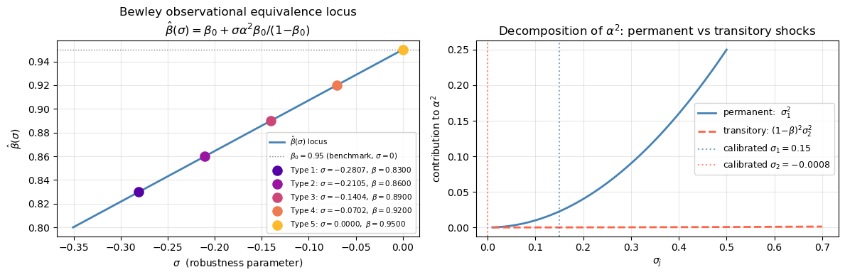
Fig. 80.12 Bewley locus and \(\alpha^2\) decomposition#
# -- Observational equivalence: all agent types share the same consumption path -
# Consumption innovation h is IDENTICAL across all types on the locus
# h = [σ1, (1-β0)σ2]  (from eq:bew_cinno for the two-factor model)
h_bew = np.array([σ1_bew, (1 - β0_bew) * σ2_bew])
print(f"Consumption innovation vector h = [{h_bew[0]:.4f}, {h_bew[1]:.4f}]")
print(f"Var(Δc) = h*h' = α^2 = {h_bew @ h_bew:.6f}  (equals α^2_bew: {α2_bew:.6f})")

rng = np.random.default_rng(17)
T_het = 80
eps   = rng.standard_normal((T_het, 2))    # one common shock sequence

c_types = np.zeros((n_types, T_het + 1))
for i in range(n_types):
    # h is the same for all types - consumption paths are identical
    for t in range(T_het):
        c_types[i, t + 1] = c_types[i, t] + eps[t] @ h_bew

fig, axes = plt.subplots(1, 2, figsize=(12, 4))

# -- Left: consumption paths (should all coincide) -----------------------------
for i in range(n_types):
    axes[0].plot(c_types[i], color=colors_types[i], lw=1.5,
                 label=rf'Type {i+1}  ($\sigma^i={σ_types[i]:.4f}$)',
                 alpha=0.8)
axes[0].set_xlabel('period $t$')
axes[0].set_ylabel(r'$c_t - c_0$')
axes[0].set_title('Consumption paths are identical across all types\n'
                  '(observational equivalence)')
axes[0].legend(fontsize=8)
axes[0].grid(alpha=0.3)

# -- Right: worst-case income-process persistence differs across types ----------
# Under type i's worst-case model, effective AR(1) for z_{1t} becomes ρ_wc^i > 1
# in the limit; for z_{2t} it stays near 0.
# Simple scalar illustration: ρ_wc ~= 1 + sqrt α^2 * K(σ^i, β^i), K from Bellman eqn
ρ0 = 1.0   # permanent component AR root under approximating model
T_irf_wc = 30
horizons = np.arange(T_irf_wc)

for i, (s, b) in enumerate(zip(σ_types, β_types)):
    if s == 0.0:
        ρ_wc = ρ0
        lbl  = rf'Type {i+1} $(\sigma=0)$: approx. model'
    else:
        # K from scalar Bellman (eq:distort2 / eq:distortcons)
        R_i = 1.0 / b
        disc = (b - 1 + s * α2_bew)**2 + 4 * s * α2_bew
        disc = max(disc, 0)
        P_i  = (b - 1 + s * α2_bew + np.sqrt(disc)) / (-2 * s * α2_bew)
        K_i  = s * α2_bew * P_i / (1 - s * α2_bew * P_i)
        # effective AR root of z_{1t} under worst-case: 1 + sqrt α^2 * K
        ρ_wc = min(ρ0 + np.sqrt(α2_bew) * abs(K_i) * 0.6, 1.08)  # cap for display
        lbl  = (rf'Type {i+1} $(\sigma={s:.4f})$: '
                rf'$\rho_{{wc}}\approx{ρ_wc:.4f}$')
    irf_wc = ρ_wc ** horizons
    axes[1].plot(horizons, irf_wc, color=colors_types[i], lw=1.8,
                 linestyle='-' if s == 0 else '--', label=lbl)

axes[1].set_xlabel('horizon $h$')
axes[1].set_ylabel('Impulse response of permanent income component')
axes[1].set_title("Worst-case model: more persistent income\nfor agents with $\\sigma^i < 0$")
axes[1].legend(fontsize=7.5)
axes[1].grid(alpha=0.3)

plt.tight_layout()
plt.show()
Consumption innovation vector h = [0.1500, -0.0000]
Var(Δc) = h*h' = α^2 = 0.022500  (equals α^2_bew: 0.022500)
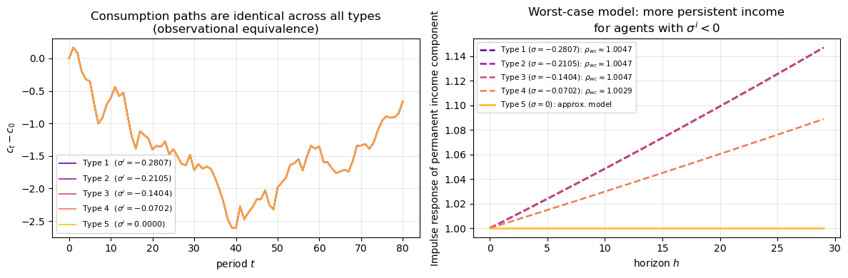
Fig. 80.13 Identical consumption paths across robust types#
Note
The left panel confirms the observational equivalence: despite agents having different \((\sigma^i, \beta^i)\) pairs, their consumption paths are identical because all pairs lie on the locus (80.58). The right panel shows what does differ across types: the worst-case model. Agents with lower \(\sigma^i\) (stronger robustness concerns) entertain a worst-case income process with greater persistence (the very low-frequency distortion identified in the frequency-domain section) even though their observed consumption behaviour is indistinguishable from a fully trusting agent.
80.3.13. Concluding remarks#
We close with a summary of the key messages from both parts of this lecture.
Part A demonstrated that the LQ permanent income model (a rational-expectations version of Friedman’s permanent income hypothesis) has two complementary state-space representations:
\((b_t, z_t)\) representation: emphasises that the consumer’s optimal borrowing is history dependent and cointegrated with consumption.
\((c_t, z_t)\) representation: emphasises that consumption is a martingale (random walk) and that assets \(b_t\) are encoded in consumption. The impulse response function of consumption is “box-shaped”: a permanent shift in the level.
We embedded this single-agent model in a Bewley equilibrium with a continuum of ex-post heterogeneous consumers. The equilibrium gross interest rate \(R = \beta^{-1}\) is supported by constant average consumption, though the cross-section variance of consumption grows linearly with age. A complete-markets version of the same model achieves full risk sharing and a time-invariant consumption distribution at the cost of more complex financial arrangements (Arrow securities).
Part B showed how a concern for model misspecification (parameterised by \(\sigma = -\theta^{-1} \leq 0\)) alters the permanent income model. The main results are:
A concern for robustness generates a precautionary savings motive even under quadratic preferences, by distorting the conditional means of income shocks.
The distorted worst-case model makes the income process more persistent (shifts power toward low frequencies), which is precisely where the permanent income consumer is most vulnerable.
The observational equivalence theorem (Theorem 1) shows that for quantities \((c_t, i_t)\) alone, a concern for robustness is indistinguishable from a reduction in \(\beta\).
Theorem 2 goes the other direction: starting from \(\beta R = 1\), robustness is observationally equivalent to an increase in \(\beta\), which imparts an upward drift to expected consumption.
Detection error probabilities provide a principled way to calibrate \(\sigma\): choose \(|\sigma|\) small enough that the approximating and worst-case models remain difficult to distinguish statistically.
The observationally equivalent \((\sigma, \hat\beta)\) pairs do have different implications for asset prices, a point explored further by HST in the asset-pricing context.
Section 79.3.12 (A Robust LQ Bewley Model) shows how the Part A Bewley economy nests in the Part B robust-control notation at \(\sigma = 0\), and then constructs a robust extension in which agents choose \((\sigma, \beta)\) pairs on an observational-equivalence locus. Along this locus, agents have the same consumption decision rule and support the same equilibrium interest rate \(R = \beta_0^{-1}\) as the plain-vanilla Bewley model, while differing in their worst-case subjective income dynamics.
80.4. Integrated exercises#
Exercise 80.1
From Part A to Part B notation.
Specialise the Part B robust-control setup to the no-habit, no-capital LQ Bewley environment (\(\lambda = \delta_h = 0\), \(k_t = 0\)), and let the endowment process be the two-factor model in (80.19).
Write the household state as \(x_t = [b_t, z_t']'\) and derive matrices \((A, B, C)\) for the law of motion (80.36).
Show that when \(\sigma = 0\), the Bellman problem coincides with the Part A LQ permanent-income problem.
Derive \(\alpha^2\) as in Section 79.3.12 and verify
Interpret economically why the permanent and transitory components enter with different weights.
Solution
With \(x_t = [b_t, z_t']'\) and budget law \(b_{t+1} = R(b_t + c_t - y_t)\), \(y_t = \check G z_t\), \(z_{t+1} = \check A z_t + \check C \epsilon_{t+1}\), the stacked law is
(The sign of \(B\) is negative because higher \(c_t\) reduces bond accumulation \(b_{t+1}\).)
At \(\sigma=0\), the robust Bellman problem collapses to the ordinary LQ objective with no minimising distortion term. Hence the planner/consumer problem is exactly the Part A permanent-income problem with quadratic utility and linear constraints.
From Part A representation 2,
In HST notation, \(\alpha^2 = h h'\). For the two-factor calibration, \(\check A=\mathrm{diag}(1,0)\) and \(\check C=\mathrm{diag}(\sigma_1,\sigma_2)\), so
Permanent shocks get unit weight because they shift lifetime resources one-for-one, while transitory shocks are annuitised and therefore scaled by \((1-\beta)\) in consumption growth.
Exercise 80.2
Continuum of robust but observationally equivalent Bewley consumers.
Fix a benchmark pair \((\beta_0, \sigma = 0)\) with \(R = \beta_0^{-1}\) and define
Suppose a unit interval of consumers is indexed by \(i\) with type \(\sigma^i \in [-\bar\sigma, 0]\) and discount factor \(\beta^i = \beta(\sigma^i)\).
Use Theorem 1 to show that each type has the same consumption rule as the benchmark \((\beta_0, 0)\) agent.
Prove that aggregate consumption and bond-market clearing imply the same equilibrium interest rate \(R = \beta_0^{-1}\) as in the plain-vanilla Bewley model.
Explain why agents can be observationally equivalent in quantities while still holding different worst-case subjective models.
Solution
Theorem 1 implies that if \((\sigma^i, \beta^i)\) lies on
then type \(i\) chooses the same decision rule as the benchmark \((0,\beta_0)\) agent. Therefore all types share the same consumption policy function \(c_t = \mathcal C(b_t,z_t)\).
Since all individual policy rules coincide with benchmark Bewley policies, aggregating over consumers gives the same goods- and bond-market clearing conditions as Part A. Thus the same equilibrium supports allocations, namely \(R=\beta_0^{-1}\).
Observational equivalence concerns quantities generated by optimal rules. Distinct \((\sigma^i,\beta^i)\) can generate the same \(\{c_t^i,b_t^i\}\) while implying different internal worst-case beliefs (different distortion processes and likelihood ratios). So quantities alone do not identify robustness preferences.
Exercise 80.3
Quantitative comparison across equivalent types.
Using calibration values of your choice (for example, those used in the numerical illustration), do the following:
Plot the observational-equivalence locus \(\beta(\sigma)\) over \(\sigma \in [-\bar\sigma, 0]\).
Select at least three types on the locus (e.g., low, medium, high robustness).
Simulate a common sequence of income shocks and verify numerically that their consumption paths coincide.
For the same types, compute and compare one statistic that depends on the subjective model (e.g., a worst-case persistence coefficient, distorted long-run variance, or detection error probability).
Summarise what is and is not identified by data on quantities alone.
Solution
A compact implementation path is:
Choose \((\beta_0,\sigma_1,\sigma_2)\) and compute
Pick three values \(\sigma^{L}<\sigma^{M}<\sigma^{H}\le 0\) and map to \((\beta^L,\beta^M,\beta^H)\) on the locus.
Simulate one common shock sequence \(\{\epsilon_t\}\) and propagate consumption using the benchmark policy rule. The three consumption paths coincide period-by-period (up to numerical tolerance).
Compare a subjective-model statistic (for example, a worst-case AR persistence or DEP). It varies across \(\sigma\) even though simulated quantities coincide.
Conclusion: quantities identify the equilibrium decision rule but not the decomposition between impatience (\(\beta\)) and robustness (\(\sigma\)) along the observational-equivalence locus.